[R 통계_ggplot2 패키지] 01-1. geom_point에 회귀선(geom_abline) 추가하기

지난 포스팅에선 geom_point 함수를 활용하여, Scatter Plot을 그려보았다.

이러한 Scatter Plot을 지나는 회귀 직선을 그리고 싶다면 어떻게 해야할까?

 

2-1. 선형 추세선 추가하기 (기본)

그래프1 <- ggplot(데이터명, aes(x축, y축)

그래프1 <- 그래프1 + geom_point()

그래프1 <- 그래프1 + geom_abline(intercept = 절편, slope = 기울기, colour = "색상")

library(ggplot2)

head(mtcars)

#회귀 값을 먼저 알아보자
lm(disp ~ mpg, data = mtcars)

<결과>
Call:
lm(formula = disp ~ mpg, data = mtcars)

Coefficients:
(Intercept)          mpg  
     580.88       -17.43  

#02-1. 회귀선 추가
plot_graph_layer1 <- ggplot(mtcars, aes(x = mpg, y = disp))
plot_graph1 <- plot_graph_layer1 + geom_point()
plot_graph_abline1 <- plot_graph1 + geom_abline(intercept = 580.88, slope = -17.43, colour = "red")
plot_graph_abline1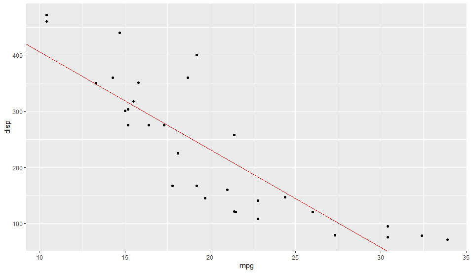

geom_point with abline

 

2-2. 선형 추세선 추가하기 (회귀 계수 값 불러오기)

그래프1 <- ggplot(데이터명, aes(x축, y축)

그래프1 <- 그래프1 + geom_point()

그래프1 <- 그래프1 + geom_abline(intercept = 계수값벡터["(Intercept)"], slope = 계수값벡터["독립변수명"], colour = "색상")

library(ggplot2)

head(mtcars)


coef <- coef(lm(disp ~ mpg, data = mtcars))
coef

<결과>  #(Intercept)와 mpg라는 변수명을 활용한다.
(Intercept)         mpg 
  580.88382   -17.42912 

#02-2. 회귀선 추가 (계수 삽입형)
plot_graph_layer2 <- ggplot(mtcars, aes(x = mpg, y = disp))
plot_graph2 <- plot_graph_layer2 + geom_point(colour="blue", size = 2 )
plot_graph_abline2 <- plot_graph2 + geom_abline(intercept = coef["(Intercept)"], slope = coef["mpg"], colour = "red")
plot_graph_abline2

geom_point with abline